Quickstart
Remote sensing data can be used for many purposes - for vegetation, climate, soil and human impact analysis. RSP can prepare raw remote sensing data for analysis.
Here is an example of some features that RSP provides. We will perform a simple task - train a semantic segmentation model that will predict landcover class using Sentinel-2 and DEM data.
First, we need to preprocess data. We preprocess Sentinel-2 images and merge them into a mosaic, then we calculate NDVI of that Sentinel-2 mosaic. We also merge DEM images into mosaic, match it to the same resolution and projection as Sentinel-2 data and normalize its values. Also, we calculate slope from DEM data. We rasterize landcover shape file and match it to the same resolution and projection as Sentinel-2 data.
Then we prepare data to semantic segmentation model training. We use Sentinel-2 and DEM data as predictors and landcover data as a target variable. We cut our data into small tiles and split it into train, validation and test subsets. Then we train and test UperNet model that predicts landcover based on Sentinel-2 and DEM data. Finally, we use this model to create a landcover map.
Importing RSP
Here we import Remote Sensing Processor
>>> import remote_sensing_processor as rsp
Sentinel-2 preprocessing
We have 6 Sentinel-2 images that cover our region of interest.
>>> from glob import glob
>>> sentinel2_imgs = glob("/home/rsp_test/sentinels/*.zip")
>>> print(sentinel2_imgs)
['/home/rsp_test/sentinels/S2A_MSIL2A_T42VWR_A032192_20210821T064626.zip',
 '/home/rsp_test/sentinels/S2A_MSIL2A_T42WXS_A032192_20210821T064626.zip',
 '/home/rsp_test/sentinels/S2A_MSIL2A_T43VCL_A032192_20210821T064626.zip',
 '/home/rsp_test/sentinels/S2A_MSIL2A_T43VDK_A031391_20210626T063027.zip',
 '/home/rsp_test/sentinels/S2A_MSIL2A_T43VDL_A023312_20210823T063624.zip',
 '/home/rsp_test/sentinels/S2A_MSIL2A_T43VDL_A031577_20210709T064041.zip']
We need to preprocess these images. Preprocessing includes superresolution for 20 and 60m bands and cloud masking.
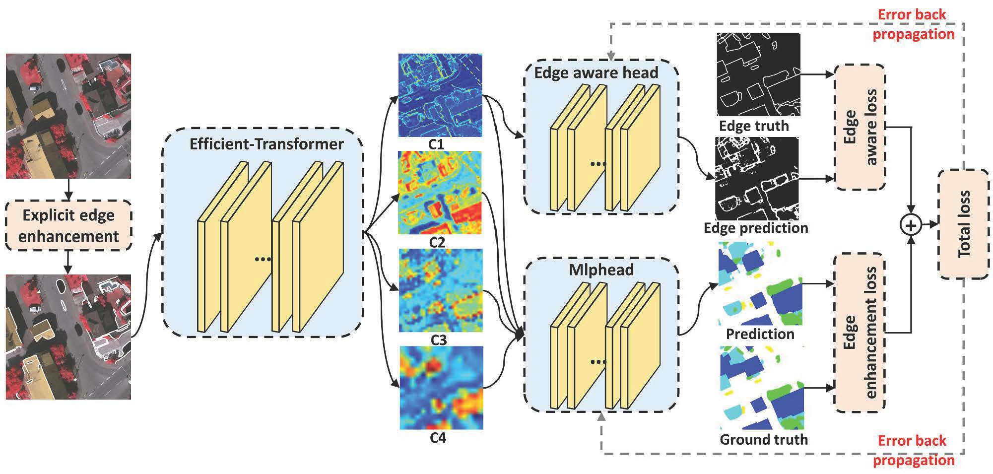
We upscale 20-m and 60-m bands to 10-m resolution with superresolution model.

Image from here
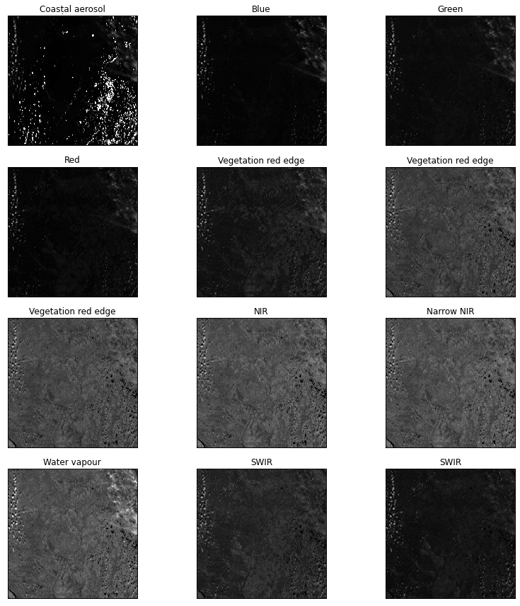
Then we mask clouds. It is done with cloud mask file from sentinel image, surface type map and with band 1 and 9 filters.
Sentinel image before masking
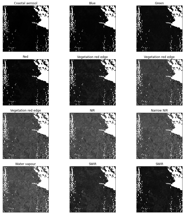
Sentinel image after cloud masking.
sentinel2 function can take list of images as input and process all of them one by one.
By default upscale is superres and cloud_mask is True, so the function will perform superresolution and mask clouds by default.
Machine learning models usually work best with normalized data, so we need to set normalize parameter to True.
>>> output_sentinels = rsp.sentinel2(sentinel2_imgs, normalize=True)
Preprocessing of /home/rsp_test/sentinels/S2A_MSIL2A_T42VWR_A032192_20210821T064626.zip completed
Preprocessing of /home/rsp_test/sentinels/S2A_MSIL2A_T42WXS_A032192_20210821T064626.zip completed
Preprocessing of /home/rsp_test/sentinels/S2A_MSIL2A_T43VCL_A032192_20210821T064626.zip completed
Preprocessing of /home/rsp_test/sentinels/S2A_MSIL2A_T43VDK_A031391_20210626T063027.zip completed
Preprocessing of /home/rsp_test/sentinels/S2A_MSIL2A_T43VDL_A023312_20210823T063624.zip completed
Preprocessing of /home/rsp_test/sentinels/S2A_MSIL2A_T43VDL_A031577_20210709T064041.zip completed
>>> print(output_sentinels)
['/home/rsp_test/sentinels/S2A_MSIL2A_T42VWR_A032192_20210821T064626/S2A_MSIL2A_T42VWR_A032192_20210821T064626.json',
 '/home/rsp_test/sentinels/S2A_MSIL2A_T42WXS_A032192_20210821T064626/S2A_MSIL2A_T42WXS_A032192_20210821T064626.json',
 '/home/rsp_test/sentinels/S2A_MSIL2A_T43VCL_A032192_20210821T064626/S2A_MSIL2A_T43VCL_A032192_20210821T064626.json',
 '/home/rsp_test/sentinels/S2A_MSIL2A_T43VDK_A031391_20210626T063027/S2A_MSIL2A_T43VDK_A031391_20210626T063027.json',
 '/home/rsp_test/sentinels/S2A_MSIL2A_T43VDL_A023312_20210823T063624/S2A_MSIL2A_T43VDL_A023312_20210823T063624.json',
 '/home/rsp_test/sentinels/S2A_MSIL2A_T43VDL_A031577_20210709T064041/S2A_MSIL2A_T43VDL_A031577_20210709T064041.json']
Function returns list of STAC files that contain metadata for preprocessed images.
Merging Sentinel-2 images
In this stage preprocessed Sentinel-2 images are being merged into one mosaic. This function can merge not only single-band images, but also multi-band imagery like Sentinel-2. fill_nodata argument makes RSP also fill the gaps in the final mosaic, clip argument is a path to a file with a border of our region of interest that is used to clip data, crs is a CRS we need, and nodata_order is to merge images in order from images with less nodata values on top (they are usually clear) to images with most nodata on bottom (they are usually most distorted and cloudy).
>>> border = "/home/rsp_test/border.gpkg"
>>> mosaic_sentinel = rsp.mosaic(
... 	output_sentinels,
... 	"/home/rsp_test/mosaics/sentinel/",
... 	fill_nodata=True,
... 	clip=border,
... 	crs="EPSG:4326",
... 	nodata_order=True,
... )
Processing completed
>>> print(mosaic_sentinel)
'/home/rsp_test/mosaics/sentinel/S2A_MSIL2A_T42VWR_A032192_20210821T064626_mosaic.json'
The function returns a STAC file with mosaic metadata.
Calculating NDVI for sentinel-2 mosaic
Normalized difference function can automatically select bands for calculating NDVI based on Sentinel-2 image, we can just give it index name and a folder where bands are stored.
>>> ndvi = rsp.calculate_index("NDVI", mosaic_sentinel)
>>> print(ndvi)
'/home/rsp_test/mosaics/sentinel/NDVI.json'
Merging DEM images
We also need to merge ASTER GDEM images into one mosaic.
>>> dems = glob("/home/rsp_test/dem/*.tif")
>>> print(dems)
['/home/rsp_test/aster_gdem/N63E069_FABDEM_V1-0.tif',
 '/home/rsp_test/aster_gdem/N63E070_FABDEM_V1-0.tif',
 '/home/rsp_test/aster_gdem/N63E071_FABDEM_V1-0.tif',
 '/home/rsp_test/aster_gdem/N64E069_FABDEM_V1-0.tif',
 '/home/rsp_test/aster_gdem/N64E070_FABDEM_V1-0.tif']
For machine learning we need our data sources to have the same CRS and the same resolution. We can match different rasters by setting reference_raster parameter. Here we set one of the Sentinel band mosaics as a reference raster.
>>> mosaic_dem = rsp.mosaic(
... 	dems,
... 	"/home/rsp_test/mosaics/dem/",
... 	clip=border,
... 	reference_raster="/home/rsp_test/mosaics/sentinel/B1.tif",
... 	nodata=0,
... )
Processing completed
>>> print(mosaic_dem)
'/home/rsp_test/mosaics/dem/N63E069_FABDEM_V1-0_mosaic.json'
Normalizing DEM mosaics
Data normalization usually can significantly improve convergence time and accuracy of neural networks, so we will normalize our data. Min/Max normalization will convert data values to range from 0 to 1. We need to set minimum value that will be 0 in normalized data and maximum value that will be 1. We know that heights in our DEM are higher than 100 m and lower than 1000 m, so we will set these values as minimum and maximum.
>>> dem = rsp.normalize.min_max(
... 	mosaic_dem,
... 	minimum=100,
...     maximum=1000,
... )
Calculating slope from DEM
Sometimes generating additional variables can improve modeling results. Let’s calculate slope from our DEM and normalize it.
>>> slope = "/home/rsp_test/dem/slope.tif"
>>> slope = rsp.dem.slope(
...     mosaic_dem,
...     output_path=slope,
...     normalize=True,
... )
Generating ML-ready datasets
The goal of this tutorial is to create a model that predict land cover classes (target variable) based on Sentinel-2 and ASTER GDEM imagery (training data). We will use Convolutional Neural Network (CNN) for this task. CNN takes tiles of same size as input and process them one by one or unite them into mini-batches.
We have a custom landcover map that we want to use to train a model. We need to rasterize it. generate_tiles function can automatically rasterize vector data. Vector files usually contain several attributes. We want to vectorize type attribute, so we set "value": "type".
Here we define x data (that will be used by CNN as input training data) and y data (that will be used as target variable).
>>> x = mosaic_sentinel + dem + slope
>>> landcover_shp = "/home/rsp_test/landcover/types.shp"
>>> y = {"name": "landcover", "path": landcover_shp, "value": "type"}
We will cut Sentinel and DEM (x) and landcover (y) data to 256x256 px tiles (tile_size = 256). To lower the bias we will random shuffle tiles (shuffle=True). To evaluate model performance on a data that was not used in model training we will split data into train, validation and test subsets in proportion 3 to 1 to 1 (split={"train": 3, "validation": 1, "test": 1}).
The function generates an ML-ready dataset in a RSPDS format (which is based on HuggingFace Datasets dataset format) and returns patch to this dataset.
>>> x_tiles, y_tiles = rsp.semantic.generate_tiles(
... 	x,
... 	y,
... 	"/home/rsp_test/model/landcover_dataset.rspds",
... 	tile_size=256,
... 	shuffle=True,
... 	split={"train": 3, "validation": 1, "test": 1},
... )
Training UperNet CNN
Here we are training UperNet CNN that predicts landcover class based on Sentinel imagery and DEM.
First, we need to set up train and validation datasets. Each dataset is a dict of 3 elements: “path”: a path to a dataset, “sub”: split name defined in generate_tiles or list of split names or ‘all’ if you need to use the whole dataset, “y”: a target varialble that you want to use. In case your dataset have only one target variable, this key can be omitted. You can provide a list of datasets to train model on multiple datasets.
>>> train_ds = {"path": dataset, "sub": "train", "y": "landcover"}
>>> val_ds = {"path": dataset, "sub": "validation", "y": "landcover"}
We will use the UperNet model architecture (model="UperNet") with ConvNeXTV2 backbone (backbone="ConvNeXTV2"). Model will be saved to /home/rsp_test/model/upernet.ckpt and could be used later for testing and prediction. Model will be trained for 100 epochs, with early stopping callback enabled and patience of 10 epochs (epochs={"max_epochs":100, "early_stopping": True, "patience": 10}) with default set of augmentations applied to train data (augment=True) and automatic selection of number of workers used (num_workers="auto").
>>> model = rsp.segmentation.train(
... 	train_ds,
... 	val_ds,
... 	model_file="/home/rsp_test/model/upernet.ckpt",
... 	model="UperNet",
... 	backbone="ConvNeXTV2",
... 	epochs={"max_epochs": 100, "early_stopping": True, "patience": 10},
...     augment=True,
...     num_workers="auto",
... )
GPU available: True (cuda), used: True
TPU available: False, using: 0 TPU cores
IPU available: False, using: 0 IPUs
HPU available: False, using: 0 HPUs
LOCAL_RANK: 0 - CUDA_VISIBLE_DEVICES: [0]

  | Name    | Type                           | Params
-----------------------------------------------------------
0 | model   | UperNetForSemanticSegmentation | 59.8 M
1 | loss_fn | CrossEntropyLoss               | 0
-----------------------------------------------------------
59.8 M    Trainable params
0         Non-trainable params
59.8 M    Total params
239.395   Total estimated model params size (MB)
Epoch 99: 100% #############################################
223/223 [1:56:20<00:00, 31.30s/it, v_num=54, train_loss_step=0.326, train_acc_step=0.871, train_auroc_step=0.796, train_iou_step=0.655,
val_loss_step=0.324, val_acc_step=0.869, val_auroc_step=0.620, val_iou_step=0.678,
val_loss_epoch=0.334, val_acc_epoch=0.807, val_auroc_epoch=0.795, val_iou_epoch=0.688,
train_loss_epoch=0.349, train_acc_epoch=0.842, train_auroc_epoch=0.797, train_iou_epoch=0.648]
`Trainer.fit` stopped: `max_epochs=100` reached.
Then we need to test model performance on test data. We will use a custom set of metrics to better evaluate model performance.
>>> test_ds = {"path": dataset, "sub": "test", "y": "landcover"}
>>> rsp.semantic.test(
...     test_ds,
...     model=model,
...     metrics=[
...         {"name": "accuracy_macro", "log": "step"},
...         {"name": "accuracy_micro", "log": "verbose"},
...         {"name": "f1_macro", "log": "step"},
...         {"name": "f1_micro", "log": "verbose"},
...         {"name": "precision_macro", "log": "step"},
...         {"name": "precision_micro", "log": "step"},
...         {"name": "recall_macro", "log": "step"},
...         {"name": "recall_micro", "log": "step"},
...         {"name": "generalized_dice_score", "log": "epoch"},
...         {"name": "mean_iou", "log": "verbose"},
...     ],
...     num_workers="auto",
... )
┏━━━━━━━━━━━━━━━━━━━━━━━━━━━━━━━━━━━┳━━━━━━━━━━━━━━━━━━━━━━━━━━━┓
┃            Test metric            ┃       DataLoader 0        ┃
┡━━━━━━━━━━━━━━━━━━━━━━━━━━━━━━━━━━━╇━━━━━━━━━━━━━━━━━━━━━━━━━━━┩
│     test_accuracy_macro_epoch     │    0.8231202960014343     │
│     test_accuracy_micro_epoch     │    0.7588028311729431     │
│        test_f1_macro_epoch        │    0.69323649406433105    │
│        test_f1_micro_epoch        │    0.6419615745544434     │
│          test_loss_epoch          │    0.40799811482429504    │
│    test_precision_macro_epoch     │    0.8231202960014343     │
│    test_precision_macro_epoch     │    0.6419615745544434     │
│      test_recall_macro_epoch      │    0.8231202960014343     │
│      test_recall_micro_epoch      │    0.6989598870277405     │
│ test_generalized_dice_score_epoch │    0.7101172804832458     │
│        test_mean_iou_epoch        │    0.6989598870277405     │
└───────────────────────────────────┴───────────────────────────┘
Mapping predictions
When we finished training a model, we can use it to create a landcover map based on its predictions. We need to define data that will be used for prediction (we will use the same dataset, but in real life it will probably be another dataset), model that will be used for predictions (it is out UperNet model) and a path where to write output map.
>>> whole_ds = {"path": dataset, "sub": "all", "y": "landcover"}
>>> output_map = "/home/rsp_test/prediction.tif"
>>> rsp.semantic.generate_map(whole_ds, model, output_map)
Predicting: 100% #################### 372/372 [32:16, 1.6s/it]